Decoding Strategies and Output Control
A language model does not write text directly. Instead, it returns logits for the next token. The decoding algorithm decides how to turn those logits into a token, and repeating this decision produces the output text.
The decoding algorithm affects the behavior of the model. Greedy decoding is deterministic and stable, but it can be dull. Sampling introduces some randomness, which can produce more diverse text but may also produce mistakes. Beam search can be useful for some constrained tasks but is usually not the best default for chat-style generation. Output constraints can make the model produce JSON or stop at a specific marker.
In this chapter, you will learn about:
- Greedy decoding
- Temperature sampling
- Top-k and nucleus sampling
- Repetition penalties
- Stop conditions
- Beam search
- Structured output constraints
Let’s get started.

Decoding Strategies and Output Control
Photo by Claudio Testa. Some rights reserved.
Overview
This chapter is divided into nine parts; they are:
- Reading Logits from a Model
- Greedy Decoding
- Temperature Sampling
- Top-$k$ Sampling
- Nucleus Sampling
- Repetition Penalties
- Beam Search
- Stop Conditions
- Structured Output Constraints
Reading Logits from a Model
The model returns a vector of logits for every position in the input sequence. For generation, you normally use only the last position because it predicts the next token.
The following example uses the Hugging Face transformers library with a small GPT-2 style model. The checkpoint is small enough for local experimentation, but the same logic applies to larger models.
|
1 2 3 4 5 6 7 8 9 10 11 12 13 14 15 16 17 18 |
import torch from transformers import AutoModelForCausalLM, AutoTokenizer
model_name = “sshleifer/tiny-gpt2” tokenizer = AutoTokenizer.from_pretrained(model_name) model = AutoModelForCausalLM.from_pretrained(model_name) model.eval()
prompt = “A language model is” input_ids = tokenizer(prompt, return_tensors=“pt”).input_ids
with torch.no_grad(): outputs = model(input_ids)
logits = outputs.logits next_token_logits = logits[:, –1, :] print(next_token_logits.shape) |
The output shape is:
The logits are not probabilities. To turn logits into probabilities, use softmax:
|
probs = torch.softmax(next_token_logits, dim=–1) |
However, you often do not need to compute probabilities explicitly. Greedy decoding only needs the index of the largest logit, which is the same as the token with the highest probability.
|
next_token = next_token_logits.argmax(dim=–1, keepdim=True) print(tokenizer.decode(next_token[0])) |
This is the simplest decoding strategy.
Greedy Decoding
Greedy decoding always chooses the token with the highest score. A complete greedy decoding function can be written as follows:
|
torch.no_grad() def greedy_decode(model, tokenizer, prompt, max_new_tokens=30): input_ids = tokenizer(prompt, return_tensors=“pt”).input_ids
for _ in range(max_new_tokens): outputs = model(input_ids) next_token_logits = outputs.logits[:, –1, :] next_token = next_token_logits.argmax(dim=–1, keepdim=True) input_ids = torch.cat([input_ids, next_token], dim=1)
if next_token.item() == tokenizer.eos_token_id: break
return tokenizer.decode(input_ids[0], skip_special_tokens=True) |
Greedy decoding is deterministic. Given the same model and prompt, it returns the same output. This is useful for debugging and for tasks where variation is undesirable.
The weakness is that the best local token is not always the best continuation. Greedy decoding can repeat itself, choose common phrases too often, and miss more interesting continuations.
Temperature Sampling
Temperature sampling draws from a probability distribution obtained by scaling the logits with a temperature parameter.
The figure below shows how temperature changes the probability distribution without changing the underlying logits. The same ten token scores are converted to probabilities three times: once with temperature 0.5, once with temperature 1, and once with temperature 2.
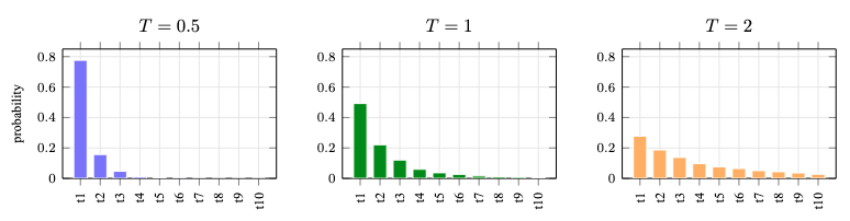
The same logits produce different token probabilities under different temperatures. A lower temperature concentrates probability on the highest-scoring token, while a higher temperature spreads probability across more tokens.
Sampling chooses the next token randomly from the model’s probability distribution. Temperature controls how sharp or flat that distribution is. Given logits $\mathbf{z}$ and temperature $T$, temperature sampling uses:
$$
\mathbf{p} = \operatorname{softmax}(\mathbf{z} / T)
$$
A low temperature makes the distribution $\mathbf{p}$ sharper. A high temperature makes it flatter. If the temperature approaches zero, sampling behaves like greedy decoding, provided one token has a uniquely highest logit. If the temperature is too high, differences between the logits become less important, and the model may choose unlikely tokens too often.
A sampling loop using temperature looks like this:
|
1 2 3 4 5 6 7 8 9 10 11 12 13 14 15 16 17 18 19 |
@torch.no_grad() def temperature_decode(model, tokenizer, prompt, temperature=0.8, max_new_tokens=30): input_ids = tokenizer(prompt, return_tensors=“pt”).input_ids assert temperature > 0, “temperature must be positive”
for _ in range(max_new_tokens): outputs = model(input_ids) # apply temperature to the logits for the next token logits = outputs.logits[:, –1, :] / temperature # convert logits to probabilities and sample from the distribution probs = torch.softmax(logits, dim=–1) next_token = torch.multinomial(probs, num_samples=1) # append the next token to the input for next iteration input_ids = torch.cat([input_ids, next_token], dim=1)
if next_token.item() == tokenizer.eos_token_id: break
return tokenizer.decode(input_ids[0], skip_special_tokens=True) |
Temperature is not a quality knob by itself. It changes the amount of randomness. The right value depends on the task. A factual extraction task usually wants a lower temperature. Brainstorming and creative writing may benefit from a higher temperature.
Top-$k$ Sampling
In the figure above, a 10-token distribution is shown as an example. An actual model may have a vocabulary of hundreds of thousands of tokens, including many that have extremely low probability in a given context.
Top-$k$ sampling keeps only the $k$ highest-scoring tokens and removes all other tokens from consideration. Its primary purpose is to prevent the model from sampling extremely unlikely tokens. It does not avoid computing logits over the full vocabulary, but it does reduce the number of candidates you sample from.
|
@torch.no_grad() def top_k_sample(logits, k): assert k > 0, “k must be positive” assert k <= logits.size(–1), “k must not exceed the vocabulary size”
# Get top-k logits and their indices values, indices = torch.topk(logits, k) # Convert logits to probabilities over top-k candidates probs = torch.softmax(values, dim=–1) # Sample from top-k indices according to their probabilities sampled = torch.multinomial(probs, num_samples=1) # Recover actual token ids using gathered top-k indices next_token = indices.gather(–1, sampled) return next_token |
Top-$k$ is easy to understand, but it uses a fixed number of candidates. Sometimes the model is very confident and only a few tokens matter. Sometimes many tokens are plausible, in which case a fixed top-$k$ cutoff may be inappropriate. This motivates nucleus sampling.
Nucleus Sampling
Nucleus sampling, also called top-$p$ sampling, keeps the smallest set of tokens whose cumulative probability is at least $p$. For example, with $p=0.9$, it keeps the most likely tokens that together account for 90 percent of the probability mass.
|
1 2 3 4 5 6 7 8 9 10 11 12 13 14 15 16 17 18 19 20 21 22 23 24 25 26 27 28 29 30 31 32 33 34 35 36 37 38 |
torch.no_grad() def top_p_sampling(logits, temperature=1.0, k=0, p=0.9): “”“ Apply temperature scaling, optional top-k filtering, and top-p filtering. Accept a 1D tensor of logits and return one sampled token ID. ““” assert logits.dim() == 1, “logits must be a 1D tensor” assert 0 < p <= 1, “p must be in (0, 1]”
vocab_size = logits.size(0)
# Apply temperature logits = logits / temperature
# Optional top-k filtering if k > 0 and k < vocab_size: topk_vals, topk_idx = torch.topk(logits, k) # Create a mask filled with -inf, put top-k logits at their indices new_logits = torch.full_like(logits, float(‘-inf’)) new_logits[topk_idx] = topk_vals logits = new_logits
# Top-p (nucleus) filtering sorted_logits, sorted_indices = torch.sort(logits, descending=True) sorted_probs = torch.softmax(sorted_logits, dim=–1) cumulative_probs = torch.cumsum(sorted_probs, dim=–1)
# Tokens to remove, but keep at least one token remove = cumulative_probs > p remove[1:] = remove[:–1].clone() remove[0] = False sorted_logits = sorted_logits.masked_fill(remove, float(‘-inf’))
# Sampling final_probs = torch.softmax(sorted_logits, dim=–1) sampled = torch.multinomial(final_probs, num_samples=1) next_token = sorted_indices.gather(–1, sampled) return next_token |
The function above combines temperature sampling, optional top-$k$ filtering, and top-$p$ filtering. Combining these techniques is common. Their order matters because temperature scaling and filtering affect the distribution from which the next token is sampled. Top-$p$ is adaptive: it may keep only a handful of tokens when the model is confident and many tokens when the distribution is broad.
Repetition Penalties
Autoregressive models can fall into loops in which a pattern of tokens repeats itself. Adding a repetition penalty reduces the scores of tokens that have already appeared so that those tokens are less likely to be chosen again.
One simple version divides positive logits by the penalty and multiplies negative logits by the penalty:
|
1 2 3 4 5 6 7 8 9 10 11 12 13 14 15 16 17 18 19 20 21 22 23 |
@torch.no_grad() def apply_repetition_penalty(logits, generated_ids, penalty=1.1): assert logits.dim() == 2 and logits.size(0) == 1, ( “logits must have shape [1, vocab_size]” ) assert generated_ids.dim() == 2 and generated_ids.size(0) == 1, ( “generated_ids must have shape [1, sequence_length]” ) assert penalty >= 1.0, “penalty must be at least 1”
if penalty == 1.0: return logits
logits = logits.clone() token_ids = set(generated_ids[0].tolist()) for token_id in token_ids: token_logit = logits[0, token_id] logits[0, token_id] = torch.where( token_logit > 0, token_logit / penalty, token_logit * penalty, ) return logits |
This function is intentionally simple and assumes a batch size of one. For example, multiple occurrences of the same token do not increase the penalty. The caller also decides whether generated_ids includes prompt tokens, generated tokens, or both. If you use repetition penalties with top-$k$ or nucleus sampling, apply the penalties first. Production implementations usually handle larger batches and may also distinguish frequency penalties from presence penalties.
Repetition penalties can help, but they can also harm quality. Some words should repeat. Code, names, citations, and structured formats often require exact repetition. Use this control only when repetition is a real problem.
Beam Search
Greedy decoding keeps only one candidate sequence. Beam search keeps several candidates. At each step, it expands each candidate with possible next tokens and keeps the best-scoring sequences.
Beam search is useful when there is a well-defined sequence-level objective, such as translation in older sequence-to-sequence systems. For open-ended chat generation, beam search often produces generic text because it favors high-probability continuations.
A minimal beam search loop looks like this:
|
1 2 3 4 5 6 7 8 9 10 11 12 13 14 15 16 17 18 19 20 21 22 23 24 25 26 |
@torch.no_grad() def beam_search(model, tokenizer, prompt, num_beams=3, max_new_tokens=20): input_ids = tokenizer(prompt, return_tensors=“pt”).input_ids beams = [(0.0, input_ids)]
# Each iteration adds one token to each beam for _ in range(max_new_tokens): candidates = [] # Expand each beam with its num_beams highest-scoring next tokens for score, token_ids in beams: outputs = model(token_ids) logits = outputs.logits[:, –1, :] log_probs = torch.log_softmax(logits, dim=–1) values, indices = torch.topk(log_probs, num_beams, dim=–1)
for value, token_id in zip(values[0], indices[0]): next_ids = torch.cat([token_ids, token_id.view(1, 1)], dim=1) candidates.append((score + value.item(), next_ids)) # Keep only the best num_beams candidates for the next iteration beams = sorted( candidates, key=lambda candidate: candidate[0], reverse=True )[:num_beams]
# Return only the best beam as the final output best_score, best_token_ids = beams[0] return tokenizer.decode(best_token_ids[0], skip_special_tokens=True) |
This implementation is deliberately small. A real implementation should normalize scores by sequence length, handle end-of-sequence tokens, and avoid recomputing the whole prefix by using a KV cache.
Beam search is expensive: the loops make generation slower, and the number of beams increases memory usage. If you use four beams, the model tracks four continuations. This increases compute and cache memory compared with ordinary sampling. Therefore, beam search is usually avoided in LLM services.
Stop Conditions
Generation must stop at some point. The simplest stop condition is a maximum number of new tokens. Another common condition is the model’s end-of-sequence token. Usually the vocabulary in a language model contains some special tokens. The end-of-sequence token is one of them.
The greedy decoding example above can be modified to accept an arbitrary stop token:
|
@torch.no_grad() def greedy_decode_with_stop(model, tokenizer, prompt, stop_token_id, max_new_tokens=30): input_ids = tokenizer(prompt, return_tensors=“pt”).input_ids
for _ in range(max_new_tokens): outputs = model(input_ids) next_token_logits = outputs.logits[:, –1, :] next_token = next_token_logits.argmax(dim=–1, keepdim=True) input_ids = torch.cat([input_ids, next_token], dim=1)
if next_token.item() == stop_token_id: break
return tokenizer.decode(input_ids[0], skip_special_tokens=True) |
This function checks whether the next token is the stop token. If it is, the loop ends and the function returns the generated text before reaching the maximum number of new tokens. This implementation does not handle batched inputs; it assumes a single prompt. With batched inputs, different sequences may stop at different times, in which case more sophisticated handling is needed.
Structured Output Constraints
Some applications need the model to produce a format such as JSON, a SQL query, or a value from a fixed list. One approach is to prompt the model and *hope* that it follows the format. A stronger approach is constrained decoding.
The idea is to mask out tokens that would make the output invalid. For example, if the output must be one of three labels, you can score only those labels:
|
1 2 3 4 5 6 7 8 9 10 11 12 13 14 15 16 17 18 19 |
@torch.no_grad() def choose_label(model, tokenizer, prompt, labels): assert labels, “labels must not be empty”
# Run the prompt to obtain logits over the vocabulary input_ids = tokenizer(prompt, return_tensors=“pt”).input_ids outputs = model(input_ids) logits = outputs.logits[:, –1, :]
# Score each label, assuming that it is exactly one token in this context label_scores = [] for label in labels: # Include any required leading whitespace in the label string label_ids = tokenizer.encode(label, add_special_tokens=False) assert len(label_ids) == 1, f“{label!r} must encode to exactly one token” label_scores.append(logits[0, label_ids[0]].item())
best_score, best_label = max(zip(label_scores, labels)) return best_label |
This example handles only labels that encode to one token after the prompt. Tokenization can depend on context, including preceding whitespace, so callers must construct the labels accordingly. Multi-token labels require scoring complete token sequences or constraining each decoding step. Structured decoding turns output requirements into token constraints. More advanced systems use grammars, tries, or finite-state machines to decide which tokens are valid at each step.
Constrained decoding can improve reliability, but it can also slow inference. The system must compute and apply token masks at each step. As with every inference technique, you should measure both quality and performance.
Further Reading
Below are some resources you may find useful:
- Softmax function, on Wikipedia.
This is a useful reference for how logits are converted into probabilities. Temperature sampling is a direct modification of the softmax input, replacing $\mathbf{z}$ with $\mathbf{z}/T$ before normalization. - Beam search, on Wikipedia.
This page describes beam search as a general heuristic search algorithm. In language generation, beam search keeps several candidate continuations instead of only the single best next token. - The Curious Case of Neural Text Degeneration, by Holtzman et al.
This paper explains why maximum-likelihood decoding methods such as greedy decoding and beam search can produce bland or repetitive text, and introduces nucleus sampling as a practical alternative for open-ended generation. - Contrastive Decoding: Open-ended Text Generation as Optimization, by Li et al.
This paper proposes a decoding method that compares an expert language model with a smaller amateur model, using the difference between their scores to prefer fluent and informative continuations. - Grammar-Constrained Decoding for Structured NLP Tasks without Finetuning, by Geng et al.
This paper discusses how formal grammars can constrain the token choices of a language model so that generated outputs follow a required structure. - Generating Structured Outputs from Language Models: Benchmark and Studies, by Geng et al.
This paper studies constrained decoding for structured outputs such as JSON schemas, and is especially relevant when the goal is reliable machine-readable output rather than free-form text.
Summary
In this chapter, you learned that decoding is the process of choosing tokens from logits. Greedy decoding is deterministic and simple. Temperature sampling, top-$k$ sampling, and nucleus sampling introduce controlled randomness. Beam search tracks multiple candidates but increases inference cost. Repetition penalties and stop conditions help control output length and behavior. Structured output constraints can make model outputs easier to use in applications.
In the next chapter, you will learn how to measure inference performance so that these choices can be compared with real numbers instead of intuition.